Interacting with the Manuscript object in Python

If you are a little savvy with Python, you can interact directly with the Manuscript in a Python interpreter. Open up the Python interpreter, Jupyter Notebook, or iPython in the manuscript-object directory and enter the following:

> from manuscript import *
> m = Manuscript(utils.ms_xml_path)

Now the Manuscript is held in memory with the variable name m. You can look at a particular entry like this:

> e = m.entries['tl']['p005r_2']

And you can inspect various aspects about it:

• e.text
• e.xml_string
• e.properties

There are also several functions which are useful when interacting with entries:

> find_terms(e.xml, "env")
['window',
 'street',
 'window',
 'window',
 'street',
 'pierced door of a closed room',
 'sun']

With a bit of Python, you can make complex queries about the manuscript this way.

> for id, entry in m.entries['tl'].items():
    if len(find_terms(entry.xml, "env")) > 0:
        print(id)
p003r_2
p003r_3
p004r_2
p004v_1
...
p169r_1
p170r_4
p170v_3

Just like that, you get a list of all the entries with environment tags in them!

If we store some data in a list, we can plot the number of env tag occurrences by entry:

> import matplotlib.pyplot as plt
> ids = []
> n_terms = []
> for id, entry in m.entries['tl'].items():
    terms = find_terms(entry.xml, "env")
    if len(terms) > 0:
        ids.append(id)
        n_terms.append(len(terms))
> plt.scatter(ids, n_terms)
> plt.show()

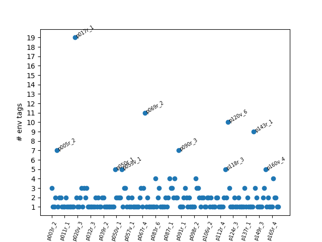
With a little extra formatting, you have a visualization of roughly where env tags appear in the manuscript!

We see that entry 17r_1 has a ton of environment tags. Why is this?

> e = entries['tl']['p017r_1']
> e.title
On the gunner
> e.properties["environment"]
['ditch casemates',
 'private houses',
 'small towns',
 'fortresses of little importance',
 'casemates',
 'trenches',
 'edge of the ditch',
 'gabions',
 'garrets topped with a tower',
 'city',
 'city',
 'barricade',
 'house or elsewhere',
 'cities',
 'houses',
 'walls',
 'tower',
 'houses',
 'houses']

So this is an entry discussing how gunners interacted with various environments in order to defend or attack them! It looks pretty long. How many characters is it?

> len(e.text)
14595

Looks like a big number, but how much is that in context?

> lengths = [len(entry.text) for entry in m.entries["tl"].values()]
> average = sum(lengths) / len(lengths)
> average
732.9827586206897

Wow! Compared to the average, this entry is super long! But that doesn’t tell us anything about the actual distribution.

> import math
> sd = math.sqrt(sum((x - average)**2 for x in lengths) / len(lengths))
> sd
1114.6637780356928

Unsurprisingly, we have a pretty significant standard deviation.

> len(e.text) / sd
13.093634410297176

So the length of entry 17r_1 is 13 standard deviations from the average entry in the manuscript!

It’s very easy to go from here to a simple histogram showing the length distribution:

> plt.hist(lengths, bins=100)
> plt.axvline(average, color="orange")
> for x in range(1,14):
    plt.axvline(average + x*sd, color="purple", linewidth=0.5)

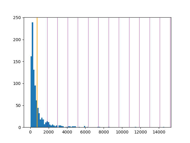
The orange line is the mean; the purple lines are standard deviations. That tiny blue blip around 14000 must be entry 17r_1.

Admittedly, this sort of statistic is not terribly informative on this kind of dataset, but possibilities are abound. Interacting with the manuscript is made simple and powerful by holding the entries in memory as a Python object.